Ligand efficiency is a widely used design parameter in drug discovery. The dependence of ligand efficiency on the concentration unit can be eliminated by defining efficiency in terms of sensitivity of affinity to molecular size and this is illustrated with reference to fragment-to-lead optimizations. An alternative to ligand efficiency for normalization of affinity with respect to molecular size is presented. The importance of examining relationships between affinity and molecular size directly is stressed throughout this study. To upgrade the contemporary In Silico drug design agenda, a novel computational version of Markov chains theory has been proposed. This is about to predict some crucial patterns of the ligand-receptor recognition and coupling.

Keywords: Ligand-target coupling; Affinity; Pharmacophores; In Silico drug design; Pharmacokinetics.

Most chemical starting points for design lack the affinity required to function as drugs and optimization typically results in increased lipophilicity, molecular size and molecular complexity [1-10]. This highlights excessive molecular size and lipophilicity as primary design risk factors. Risks associated with molecular complexity [2,6,9] are more likely to be encountered in the screening phase of a project. Molecular complexity can also be seen inversely as the degree to which a compound is structurally prototypical [1,3,7] (e.g., minimally substituted) and might also be defined in terms of the molecular shape [7,10] of a compound or the roughness [8,10] of its molecular surface. Molecular recognition [1,5,9] provides much of the conceptual framework for drug design and many medicinal chemists consider molecular interactions [6,9,10] when elaborating chemical start points. While a structure-activity relationship can point to the importance of individual interactions, the contribution of a protein-ligand contact to affinity is not, in general, an experimental observable [1-9].

It would be safe to say, however, that a weak link in a row of the drug design leading events is a hard way to make a choice of the most efficient pharmacophore revealed within a paradigm of the «drug-target», i.e. «ligand-receptor», affinity docking. To optimize a solution of this dilemma, an arsenal of mathematical methods might be employed once they’re focused on a modeling and testing of the above mentioned phenomena.

As per these methods themselves, they are still far of being perfect and yet there is «enough room ahead» to move forward with an attempt to upgrade the current probabilistic computational outlook for better In Silico ligand-receptor fitting. This attempt our present study is all about.

Bailey differential equation

Legible proof of Bailey’s formula [2,3,8] is presented in this work in a form suited for immediate practical use. Below stands for time and x(t),t ≥ 0 denotes a homogeneous Markov chain with continuous time and the state space N_o consisting of non-negative integers (the population, in the basics example considered). The process values x(t) at time are denoted as {x(t)}, and ∆x(t)=x(t+∆t)-x(t) is the Markov process increment (the population change over the period of time from t to t+∆t) The probability distribution at time is determined by the probabilities P_x(t) of the population numbering x(t) species at time t.

The probability-generating function of the distribution for the process x(t) is given by

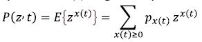
with |z|≤1. The transition function for the Markov process is defined by the probability distribution for ∆x(t). For a homogeneous Markov chain (provided that the transitions occur), we have, up to infinitesimal corrections

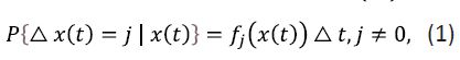
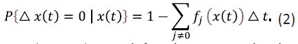
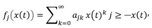
where the transition intensities f_j(x(t)) are non-negative functions depending solely on x(t) for fixed values of . It should be noted that, since the set of states x(t) for the process considered is comprised of non-negative numbers, the reasonable assumption is that f_j(x(t))≐0 for j<-x(t).

In this case, the probability that no transition occurs betweenIn this case, the probability that no transition occurs between t and t+∆t is, up to an infinitesimal term given by

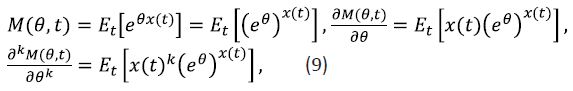
Let E_t(g(x(t))) stand for the expected value of g(x(t)) at time, t, g(u) with u≥0 being a measurable function; let E_t+∆t(g(x(t+∆t))) g(x(t)) at t+∆t; and let E_t/∆t {g(x(t+∆t)|x(t))} be the conditional expectation for g(x(t+∆t). Also, assume that M (θ , t) = E_t{e^θx(t)}=P(e^θ , t) with θ < 0 is the Laplace-Stieljes transform of the probability distribution for process x(t) which is designated as the moment-generating function; K(θ , t) = In M (θ, t) is the cumulant-generating function. The cumulant-generating function is customarily represented in the form of Taylor series in θ

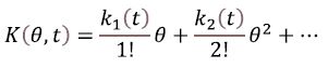
Here is the i-th cumulant of the x(t) process at time t ≥ 0 The first cumulant is equal to the expected value, the second – to dispersion, and the first cross-cumulant – to covariance.

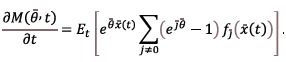
Theorem 1. Suppose the above homogeneous Markov chain x(t), t≥0 with continuous time and with the state space is defined and its generating function M (θ, t) is differentiable. Then the generating function of the homogeneous Markov process is governed by the equation

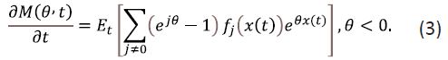
Proof 1: Assuming that all of the expected values implied below exist, the expected value obeys the relation

Given the above and as long as the expected values exist and the process is of the Markov type, the moment-generating function for the process x(t), t≥0 at time t+∆t can be written with the help of Eq. (4) as

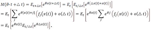
Therefore,

Therefore,

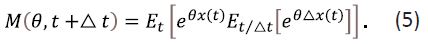
Thus,

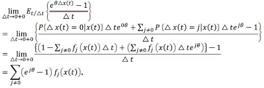
3. The derivative of the moment-generating function exists and

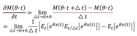
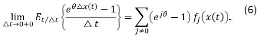
Since exists and depends on f_j(x(t)) according to Eq. (6),

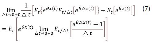
Theorem 1 follows from Eqs. (6) and (7).

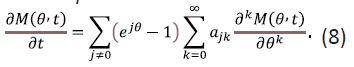
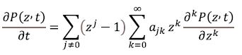
Theorem 2. If, for the above homogeneous Markov chain with x(t), t≥0 with continuous time, and with the state space N₀ the functions f_j(x(t)) can be presented as polynomials of the form

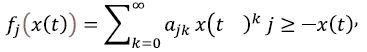
and if the derivatives implied below exist, the following differential equation holds true

Proof. Taking into account that

Eq. (1-3) can be cast in the form

which proves the theorem.

Theorem 3. If, for the above homogeneous Markov chain with , with x(t), t≥ 0 continuous time, and with the state space N₀ the functions fj(x(t)) can be presented as polynomials of the form

and if the derivatives implied below exist, the following differential equation holds true

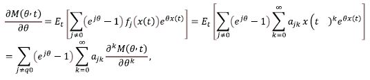
Theorems synergic proccessing. Given that the derivatives exist and that M (θ, t) = P(e^θ, t) the change of variables from to e^θ yields

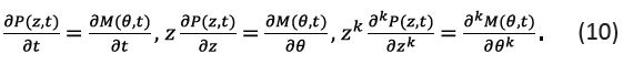
The left-hand sides of the above expressions exist, meaning that so do the corresponding right-hand sides. Consequently, the requirements of Theorem 2 are met. Substituting Eqs. (1-10) into Eq. (8), one arrives at the result stated by Theorem 3.

The approach stemming from the above derivations is that the differential equation for the moment-generating function can be spelled out directly when the functions f_j(x(t)) are available. The practical applications of the above differential equations are examined below.

Application of outcomming algorithms.

1. Suppose that a two-dimensional homogeneous Markov chain (x(t), y(t)), t≥0 with the state space (N₀xN₀) and continuous time is treated and that, similarly, the transition intensities are non-negative functions such that 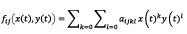. Then, if the pertinent derivatives exist, Eq. (8) affords the following generalization

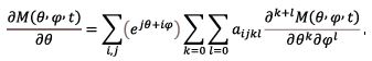
2. Consider a multidimensional Markov chain x(t) = {x₁(t),x₂(t),...,x_n(t),...}, t≥0 with continuous time and the state space N = {N₀xN₀x...N₀x...,} and denote θ = {θ₁, θ₂,...,θ_n,...}, j = {j₁,j₂,...,j_n,...}. It can be demonstrated that, sssprovided that the pertinent expected values and derivatives exist, in the general case Eq. (3) translates into the vector equation

First-order elementary chemical reaction:

Suppose that the process of decay of substance A paralleled by the generation of substance B evolves with the probability α per molecule: The process is described by the function f_-1 = αt, and Bailey’s equations become

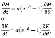
or, alternatively

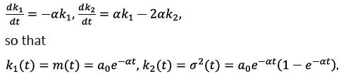
Here a₀ is the initial concentration of A, assuming that the initial dispersion of A is zero.

For the simplest reversible reaction the formation of B is described by f1 = a(a₀-x) and the decomposition – by f_-1 = βx, x being the random number of molecules of B. The corresponding Bailey’s equation is

or

Ligand-receptor interaction

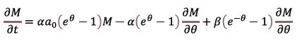
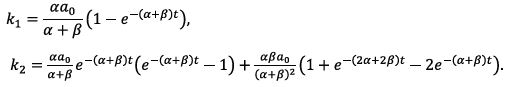
Consider a ligand-receptor interaction where R is the receptor, L is the ligand, RL is the ligand-receptor complex, α is the probability of formation of a complex molecule, and β is the probability of its dissociation. If the random number of ligand-receptor complex molecules is R₀, and the initial number of receptors is , the number of free receptors makes R_O - x. Assume that the process unfolds under the condition of large ligand surplus, so that the number of ligand molecules stays equal to its initial value L₀. The formation of ligand-receptor complexes is described by the function f₁ = αL₀(R₀ - x), and their decomposition – by f_-1 = βx. Bailey’s equation for the case is

or

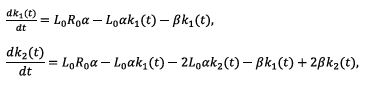
or

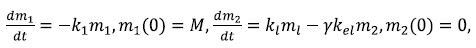
Pharmacokinetic outlook: A pharmacokinetic model of the dependence of drug concentration on time is used to gain insight into the temporal character of the emergence of dose-response relationships, the underlying assumption being that the drug is administered per os. In the simplest case, the process is described by the single-compartment model:

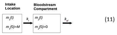
Here m₁(t) is the drug mass at the intake location, m₂(t) s the drug mass in bloodstream,k₁ and k_el are the rates of drug administration and elimination from blood. The conditions that the drug is initially localized where it is being introduces are expressed as

m₁(t) = 0, m₂(t) = M (12)

The law of mass action for scheme (11) and Eq. (12) is

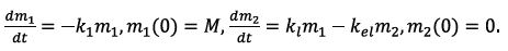
The solution to the above set of equations is (13)

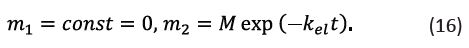
An analogous set of equations for a drug directly injected into the bloodstream is

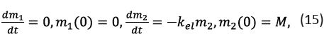
its solution trivially being

The forms of the solutions to Eqs. (13) and (14) are impractical, considering that the drug concentration in the bloodstream rather than its total mass is typically measured experimentally. Eqs. (13) and (14) can be conveniently transformed using the fact that drug concentration and mass m are related as

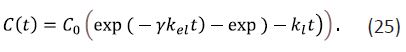
where is the blood volume. The latter may actually change due to a range of factors such as, for example, the use of diuretics. However, it can be assumed if the drug does not affect diuresis that V = const ≃ 5L. Then, the combination of Eqs. (14) and (17) results in

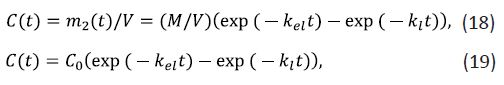
where C(t) is the time-dependent drug concentration in the bloodstream and is a constant denoting its initial effective concentration. The C₀ is a constant denoting its initial effective concentration. The drug concentration increases initially and subsequently decreases.

If the drug is directly injected into the bloodstream, the solution is more compact than the one defined by Eqs. (18) and (19)

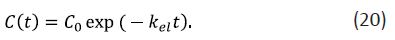
The latter expression shows that in this case the drug concentration in the bloodstream decreases monotonously.

Importantly, the majority of drugs in blood bind to transport proteins rather than stay in free state. The formation of the complex involving transport protein is described by the scheme

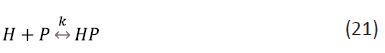
where 𝐻 is the drug, 𝑃 is the blood protein, 𝐻 𝑃 is their complex, and K is the dissociation constant.

The drug concentration generally tends to be much lower than that of the blood proteins. For example, the concentration of albumin, which is the key binding blood protein, is 10-5 M while the concentration of the nerve growth factor only reaches 10-9-10-11 M [11, 12]. The concentration of the growth hormone is 0.5-2.0 nM [13, 14] while the concentration of the binding protein is 1.5 mM [11-14]. Therefore, the concentration of the drug-blood protein complexes for scheme (21) is

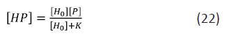
where [H₀] s the initial concentration of the drug. For most drugs, K ≫ [H] and, accordingly, Eq. (22) becomes

[H P ] = α[H₀]

with α = [P ]/K. Then, the drug concentration is

where β is the binding constant. The value β = 1 means that the drug undergoes no binding with blood proteins, and β = 0 shows that all drug molecules are drawn into association with blood proteins.

It may be the case that only bound drug (e.g. bilirubin) or only unbound agent (e.g. sex steroids) is excreted. In this situation, Eq. (23) is rewritten as

where γ is a constant such that γ = α if only the bound form of the drug is excreted and γ = β the opposite case. The solution to Eqs. (14-24) is

It should be noted that the underlying assumption in the analysis of biological effects which are due to the evolving drug concentration on the basis of Eq. (14-25) is that only the free form of the drug triggers response.

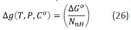
Compound-level efficiency metrics are typically constructed by either scaling (i.e., divide affinity by risk factor) or offsetting (i.e., subtract risk factor from affinity) [2-7]. LE was introduced [1,8,11] as a metric to normalize affinity with respect to molecular size by scaling the standard free energy of binding, , by the number, N_nH of non-hydrogen atoms (the term heavy atoms is also used) in the molecular structure as follows:

The standard state was not specified when the LE metric was introduced although it appears to be widely believed [15] that C° must be set to 1 M for calculation of LE. The Achilles heel of the LE metric is its nontrivial dependency [16] on C° and, as conventionally [3,7] defined, LE has a 1 M concentration unit built into it. As noted in [5,6,17] the choice of a particular value of C°, such as 1 M, to define the standard state is entirely arbitrary and a requirement that C° only take a specific value cannot be accommodated within the framework of thermodynamics. This means that LE cannot be defined objectively in absolute terms for individual compounds because there is no physical basis for favoring a particular value of C° for calculation of LE.

Drug design guidelines are typically based on trends observed in data and the strengths of these trends indicate how rigidly guidelines should be adhered to. While excessive molecular size and lipophilicity are widely accepted as primary risk factors in drug design, it is unclear how directly predictive they are of more tangible risks such as poor oral absorption, inadequate intracellular exposure and rapid turnover by metabolic enzymes. This is an important consideration because the strength of the rationale for using LE depends on the degree to which molecular size is predictive of risk. Drug discovery scientists need to be wary of correlation inflation [3-8,18] which can be loosely defined as presentation or analysis of data in any way that makes trends appear to be stronger than they actually are. Correlation inflation is a particular concern when analysis of proprietary data is presented in support of a view that a set of guidelines is especially useful or predictive.

The relevance of data must also be considered when using physicochemical characteristics such as molecular size to assess risk. For example, an activity threshold [4,19] of > 30% inhibition at 10 μM for promiscuity analysis is not especially relevant if considering the likelihood of off-target effects for a drug with a peak unbound plasma concentration of 100 nM. Sample bias can be significant, even in large datasets, as exemplified by divergent conclusions of two apparently similar studies [7,10] with respect to the relationship between pharmacological promiscuity and molecular size. The observation that average molecular weight appears to decrease [1,9] with promiscuity is particularly relevant to the use of LE because promiscuity would generally be considered [8,20-22] to be an undesirable characteristic for a compound. Drug designers should not automatically assume that conclusions drawn from analysis of large, structurally-diverse data sets are necessarily relevant to the specific drug design projects on which they are working.

The LE metric [4-10] was introduced in thermodynamic terms and it is sometimes believed that it measures the degree to which molecular interactions between ligand and target are optimal.

The standard free energy of binding, ΔG⁰ [7,10] can be written in terms of the gas constant (R), thermodynamic temperature (T), C° and the equilibrium concentrations of protein ([P]), ligand ([L]), and protein-ligand complex ([P.L]):

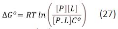
Equation (27) shows that ΔG⁰ is a function of C° and this is one reason that values of standard free energy of binding should not be termed absolute. By convention, C° is taken to be 1 M although, this is arbitrary and the value of C° has no physical significance [6-9]. In thermodynamic analysis, a change in perception resulting from a change in a standard state definition would generally be regarded as a serious error rather than a penetrating insight. In some situations, the dissociation constant, K₀, is defined to be equal to the argument of the logarithm in equation (27) and is therefore dimensionless. However, in medicinal chemistry, biochemistry and biophysics, k₀ values are conventionally quoted in units of concentration and equation (27) can be written as:

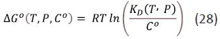
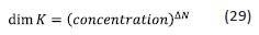
Equation (28) shows that a tenfold increase in C° leads to a decrease in ΔG⁰ of 1.36 kcal/mol at 298 K. The sign of ΔG⁰ has no special significance and simply indicates whether or not K₀ is greater or less than C°. The dependence of ΔG⁰ on C° is a consequence of the stoichiometry of association of ligand with target and ΔG⁰ for formation of a ternary complex (relevant when considering the thermodynamic consequences of fragment linking) will exhibit a different dependence on C° to ΔG⁰ for a binary complex. The stoichiometry corresponding to a ΔG⁰ value is specified by the change, ΔN, in the number of species for the corresponding reaction and it can also be seen as a ‘hidden dimension’ of ΔG⁰ For example, formation and dissociation of 1:1 complexes have ΔN values of –1 and +1 respectively. The value of ΔN determines the dimensions of the corresponding equilibrium constant:

The dependence of ΔG⁰ on C° is a consequence of the loss of translational entropy resulting from association and it has two important implications. First, ratios of ΔG⁰ values also depend on C° even though the ratios themselves are dimensionless and ΔG⁰ values should therefore be compared as differences (i.e., ΔΔG) Second, if a free energy change is written as a sum of free energy changes then the sum needs to have the same dependency on C° as the original free energy change since the equality must hold for all values of C°. This is equivalent to requiring that the sum of ΔN values for the components of a free energy decomposition be equal to the ΔN, value for the free energy change that is decomposed.

One way in which stoichiometry can be accounted for in free energy decompositions is to associate each free change with its corresponding ΔN value using square brackets. The study on attribution and additivity of binding energies can be used to illustrate this: the intrinsic binding energy for a group X as the difference in ΔG⁰ for compounds in which X is present (AX) or absent (A) in the relevant molecular structures:

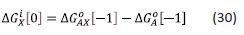
The intrinsic binding energy is associated with a zero value of ΔN and is therefore independent of C°. It shows the ΔG⁰ value for a compound with linked groups A and В in its molecular structure as the sum of the intrinsic binding energies of A and B, and the “connection Gibbs energy” (ΔG^S):

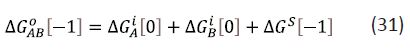
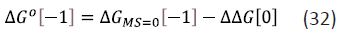
Equation (31) is particularly relevant to fragment linking and it is important to note that ΔG^S does depend on C° [1, 2]. In some studies, ΔG⁰ is decomposed into a value corresponding to zero molecular size (ΔG_{MS = 0}) and a ΔΔG value [5,9]:

One general approach to modelling affinity is to use equation (33) in which A_i (i > 0) is a parameter associated with the substructure i and ni is the number of occurrences of that substructural element:

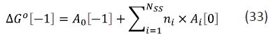
The A0 term has the same dependency on C° as ΔG⁰ and its inclusion in equation (33) allows changes in concentration unit to be easily accounted for. The substructures are typically groups at substitution sites on a scaffold and the ni values are either 1 or 0 and A₀ may correspond to the affinity of the unsubstituted scaffold.

Schemes for decomposition of ΔG⁰ based on equation (33) cannot be considered to be group additive because of the presence of the A₀ term which is not associated with any group.

An equivalent way to examine the stoichiometry issue is to consider the implications of writing K_D as follows where K_nH corresponds to Δg as defined in equation (26):

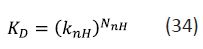
Consider two compounds X (K_D = 10-3 M; N_nH = 10) and Y (K_D = 10-6 M; N_nH = 20) that would usually be considered to be equally ligand-efficient (Δg = 0.4 kcal/mol per non-hydrogen atom at 298 К for C° = 1 M). While the values of k_nH calculated for X (0.501 M^0.1) and Y (0.501 M^0.05) have the same numerical value, it is incorrect to equate them because their dimensions differ, as reflected by the difference in their respective units. If K_D is expressed in millimolar units, the numerical values of K_nH for X (1 mM^0.1) and Y (0.708 mM^0.05) are no longer identical.

Some of the entropy of binding results from molecular interactions (e.g., between water molecules) that are non-local with respect to protein-ligand contacts. Some contributions to binding enthalpy, such as the enthalpic penalties associated with ligand and target adopting their bound conformations are also inherently non-local. A less obvious example of a non-local effect would be substitution at one position of a molecular structure preventing a substituent at another position from forming optimal interactions with the target. When interpreting binding thermodynamics in terms of molecular interactions, it should always be kept in mind that intermolecular contacts (e.g., between unbound ligand and solvent) that are not present in the protein-ligand complex also influence ΔH and ΔS⁰

Some of the problems that result from using LE as a design metric can be seen more clearly if it is expressed using a base 10 logarithm and without energy units:

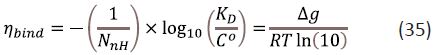
The quantity η_bind is related to Δg by a multiplicative factor of RTln (10) that is independent of C° and therefore both quantities respond in an identical manner to a change in C°. One rationale for using η_bind is that drug discovery scientists typically use pIC₅₀ or pK_D rather than ΔS⁰ in «drug-target» analysis. The quantity η_bind is also related to Ligand Efficiency by Atomic Number (LEAN) that is calculated by scaling pIC₅₀ by N _nH Unlike LEAN, η_bind is a function of C° and can also be written as η_bindC⁰ to emphasize this. Although standard state conventions do not apply to potency measures such as IC50 and EC₅₀, which are usually quoted in μM or nM, potency must still be scaled by a concentration value for the logarithm calculation because the logarithm function is not defined for dimensioned quantities. Using η_bind rather than ΔG⁰ reinforces the point that the problems associated with LE are due to the mathematical behavior of the logarithm function. While the use of a concentration unit other than 1 M to define LE is unusual, there certainly is precedent for doing so.

LE is used to specify affinity cutoffs as a function of molecular size and a Δg value of 0.3 kcal/mol per non-hydrogen atom has been suggested [6,10]. Specification of affinity cutoffs in this manner forces the line defining acceptable affinity to intersect the affinity axis at a point corresponding to a K_D value of 1 M. The minimum Δg value of 0.12 kcal/mol per non-hydrogen atom recommended can be translated (C° = 1 M; T = 300 K) to рК_D values corresponding to the lower (700 Da; N_nH ≈ 50) and upper (3000 Da; N_nH ≈ 214) limits. The lower (pK_D= 4.4) of these two values would not appear to be a useful design criterion while the higher value (pK_D= 18.7) would not generally be measurable. In general, affinity thresholds should be specified directly and LE should only be used for this purpose if supported by the data.

LE features prominently in the literature of fragment-based lead discovery [7,20,21] to the extent that it is sometimes presented as an important rationale for screening fragments.

Comparison of LE values for fragment hits and the corresponding leads can be seen as an attempt to quantify how effectively an increase in molecular size translates to affinity. This is still a valid objective even though the LE metric would appear to be unfit for this purpose. The most obvious way to do this is to scale ΔpK_D by ΔN_nH

Using ΔpK_D (the logarithm of a ratio of K_D values) eliminates the dependency on C° that makes η_bind (and Δg) unsuitable for comparison of start and end points for projects. An additional benefit is that ΔpK_D is likely to be relatively insensitive to the approximation of K_D by IC50. This approach to assessing optimizations has precedent [4] and reported that a tenfold improvement in K_D corresponded to a mean increase in molecular weight of 64 Da (standard deviation = 18 Da) for 73 compound pairs. Some other reports [3,8,10] also illustrates the benefit of observing the response of affinity to an increase in molecular size directly rather than indirectly by using the LE metric.

It can be useful to compare the changes in affinity and lipophilicity that result from structural elaboration and one way of achieving this is to offset the change in affinity by change in lipophilicity:

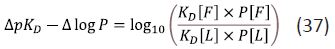
The quantity in equation (37) may be regarded as a measure of the lipophilicity efficiency. It is desirable that it should be as large as possible most drug design cases studied. Variations of equation (37) can also be written using potency (e.g. pIC50) with a measured distribution coefficient (logD) or a predicted value of logP.

Observation that a small structural change leads to a large change in affinity is usually informative. Group Efficiency (GE) is defined for the addition of a group, X, to A by scaling the value of the associated ΔΔG (ΔGⁱ_xas defined in) by ΔN_nH:

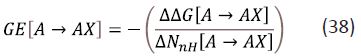
The notation [XY] can be used to specify structural transformations and to indicate that a change in the value of a property such as ΔG⁰, pK_D or N_nH has been calculated by subtracting the value of the property for compound X from that for compound Y. The definition of GE expresses equation (36) in terms of free energy rather than dissociation constant and equation (37) could be used in an analogous manner to specify the efficiency of substitutions from the perspective of lipophilicity. The fundamental difference between the two metrics is that GE is independent of C° because it is defined in terms of ΔΔG. Although GE is sometimes presented as a substructural (e.g. chloro substituent) property, it is actually structural transformations (e.g. substitute hydrogen with chlorine) with which values of GE should be associated. The ΔΔG. values used for calculation of GE cannot generally be interpreted as substructural contributions to affinity because summation of values of ΔΔG (ΔN = 0) cannot reproduce the dependency of ΔG⁰(ΔN = -1) on C°.

Drug discovery scientists typically need be able to address a range of questions when interrogating project data. For example, it may be useful to focus analysis on the most active compounds in an optimization project. It is important to stress that residuals are not generated in isolation and they result from analysis that, arguably, should be performed anyway. The line fit to a plot of affinity against molecular size is likely to be a better predictor of outcome than a line that has been artificially forced to intercept the affinity axis at a point corresponding to a K_D value of 1 M. The strength of the trend also provides an indication of how useful normalization of the data is likely to be. For example, the observation of a very weak correlation between affinity and molecular size for hits from a fragment screen suggests that molecular size need not be accounted for when assessing the fragment hits in question. In an optimization project, a relatively weak correlation between affinity and molecular size may point to the extent that it cannot be adequately explained by molecular size alone.

A neglected Baileyan computational approach is now modified to renovate and improve the In Silico pharmacokinetic modeling suitable for either preclinical trail planning or the drug- receptor docking scenaria analysis. This was found a promising research tool for the «drug-target» interaction analysis required by a contemporary drug design paradigm.

LE has been discussed in depth from a physicochemical perspective in this study and the difficulty of interpreting affinity in terms of molecular interactions was highlighted. The nontrivial dependency of LE on the concentration unit in which affinity is expressed means that LE has no physical significance and, strictly, should not even be considered to be a metric. As such, LE is unsuitable for ranking compounds, setting acceptability thresholds for affinity and modeling relationships between affinity and molecular size. While it does not appear to be possible to quantify efficiency of binding objectively for compounds in an absolute manner, efficiency can still be defined in a relative manner by scaling affinity differences by the corresponding molecular size differences.

Abbreviations: C°: standard Concentration, GE: Group Efficiency; IC₅₀: half maximal inhibitory concentration; K_D: dissociation constant; LE: Ligand Efficiency; logD: base 10 logarithm of octanol/water distribution coefficient; logP: base 10 logarithm of octanol/water partition coefficient; N_nH: number of non-hydrogen atoms in a molecular structure; P: octanol/water Partition coefficient; pIC₅₀: –log₁₀(IC50/M); pK_D: –log₁₀(pKD/M); pK_D[expt]: experimentally measured pK_D; pK_D[pred]: value of pK_D predicted by model; pK_D[resd]: residual рК_D; R: gas constant; T: thermodynamic temperature; TIP: Target Interaction Potential; Δg⁰: ligand efficiency calculated from standard free energy of binding; Δg⁰: standard free energy of binding; ΔN: change in number of chemical species; η_bind: ligand efficiency calculated from logarithmically expressed K_D without energy units.

Acknowledgements: Authors are grateful to Dr. Santiago Camacho (Dept. Mathematics and Computer Science, Wesleyan University - Bloomington, IL) for stimulating comments on preliminary findings.

1. Muro S. Challenges in design and characterization of ligand-targeted drug delivery systems. J. Controled Release. 2012; 162(2): 125-137.
2. Wang Y, Zeng J. (2013) Predicting drug-target interactions using restricted Bolzman machines. Bioinformatics. 2013; 29(1): 126-134.
3. Pawson AJ, Sharman JL, Benson HE, Faccenda E, Alexander SPH, et al. The IUPHAR/BPS Guide to pharmacology: An expert - driven knowledge base of drug targets and their ligands. Nucleic Acids Research. 2014; 42(D1): D1098 - D1106.
4. Salahudeen MS, Nishtala PS. An overview of pharmacodynamic modelling, ligand-binding approach and its application in clinical practice. Saudi Pharm J. 2017; 25(2): 165-175.
5. Li D, Ji B. Protein conformational transitions coupling with ligand interactions: Simulations from molecules to medicine. Medicine in Novel Technology and Devices. 2019; 3(6): 100026-100038.
6. Hoize J, Bermudez M, Pfeil EM, Kauk M, Bodefeld T, et al. Ligand-specific allosteric coupling controls receptor signalling. ACS Pharmacol. Transl. Sci. 2020; 3(5): 859-867.
7. Zhu S, Wu M, Huang Z, An J. Trends in application of advancing computational approaches in ligand discovery. Exterimental Biology and Medicine. 2021; 246(9): 1011-1024.
8. Farinde A. Drug - Receptor Interactions. South California University Press: Orange Beach, CA. 2022.
9. Le J. Overview of Pharmacokinetics, University of California Publ.; San Diego, CA. 2022.
10. Saurabh S, Nadendla K, Purohit SS, Sivakumar PM, Cetinel S. Fuzzy drug targets: disorded proteins in the drug-discovery realm. ACS Omega. 2023; 8(11): 9729-9747.
11. Braga E, Baik H, Lee D, Sturmer R, Heuer J, et al. Synthesis of human TFF1, its homodimer provides novel insights into mechanisms of action. Chemical Communications. 2020; 56 (47): 6420 - 6423.
12. Muttenhaler M, King GF, Adams DJ, Alewood PF. Trends in peptide drug discovery. Nature Reviews Drug Discovery. 2021; 20(4): 309-325.
13. Angelopoulou E, Pyrgelis ES, Piperi C. Emerging potential of the PDE inhibitor ibudilast for neurodegenerative diseases: an update on preclinical and clinical evidence. Molecules. 2022; 27(23): 8448-8454.
14. Sijben HJ, Superti-Furga G, Jjzerman AP, Heitman L. Targeting solute carriers to modulate receptor - ligand interactions. Trends in Pharmacological Sciences. 2022; 43(5): 358-361.
15. Zastrow M. Drug Receptors & Pharmacokinetics.14th Edition (Katzung BG, Ed.). McGraw Hill Medical Publ.: Maidenhead, UK. 2017; 260 -283.
16. Bazzari FH, Bazzari AH. BACE1 inhibitors for Alzheimer’s Disease: The past, present and any future? Molecules. 2022; 27(24): 8823-8832.
17. Lazewska D, Olejarz - Maciej A, Reiner D, Kaleta M, Latacz G, et al. Dual target ligands with receptor antagonists and monoamine oxidase B inhibitors. Int. J. Mol. Sci. 2020; 21(10): 3411-3418.
18. Poongavanam V, Kolling F, Giese A, Goller AH, Lehman L, et al. Pedictive modeling of PROTAC cell permeability with machine learning. ACS Omega. 2023; 8(6): 5901-5916.
19. Yang D, Zhou Q, Labroska V, Qin S, Darbalaei S, et al. G protein - coupled receptors: structure-and function-based drug discovery. Signal Transduction and Targeted Therapy. 2021; 7(1): 26-38.
20. Babcock JJ, Li M. Inside job: Ligand - receptor pharmacology beneath the plasma membrane. Acta Pharmacologica Sinica. 2013; 34(7): 859-869.
21. Nasser TA, Adel R, Badr A, Teleb M, Bekhit AA, et al. Combined cancer immunotheranostic nanomedicines: Delivery technologies and therapeutic outcomes. ACS Omega. 2023; 8(7): 4491-4507.
22. He X, You C, Jiang H, Xu HE, Cheneg X. Evaluation on G protein-coupled receptors. Acta Pharmacoloêica Sinica. 2023; 44(1): 1-7.